Missing Data (part one)

Over the next few weeks I’m going to be discussing some aspects of missing data. This is an important aspect of chemometrics as many applications suffer from this problem. Missing data is especially common in process applications where there are many independent sensors.

I got interested in missing data while in graduate school in the late 1980s. I worked a lot with a prototype glass melter for the solidification of nuclear fuel reprocessing waste. The primary measurements were temperatures provided by thermocouple sensors. The very high temperatures in this system, nearing 1200C (~2200F), caused the thermocouples to fail frequently. Thus it was common for the data record to be incomplete.

Missing data is also common in batch process monitoring. There are several approaches for building models on complete, finished batches. However, it is most useful to know if batches are going wrong BEFORE they are complete. Thus, it is desirable to be able to apply the model to an incomplete data record.

Missing data problems can be divided into two classes: 1)those involving missing data when applying an existing model to new data records, and 2) those involving building a model on an incomplete data record. Of these, the first problem is by far the easiest to deal with, so we will start with it. It will, however, illustrate some approaches which can be modified for use in the second case. These approaches can also be used for other purposes as well, such as cross-validation of Principal Component Analysis (PCA) models.

Consider now the case where you have a process that periodically produces a new data vector x_i (1 x n). With it you have a validated PCA model, with loadings P_k (n x k). The residual sum-of-squares or Q statistic, can be calculated for the i^th sample as Q = x_iRx_i‘ where R = I–P_kP_k‘. For the sake of convenience, imagine that the first p variables in this model are no longer available, but the remaining n–p variables are as usual. Thus, x can be partitioned into a group of bad variables x_b and a group of good variables x_g, x = [x_b x_g]. The calculation of Q can then be broken down into parts which do and do not involve missing variables:

Q = x_bR₁₁x_b‘ + x_gR₂₁x_b‘ + x_bR₁₂x_g‘ + x_gR₂₂x_g‘

where R₁₁ is the upper left (p x p) part of R, R₁₂ = R₂₁‘ is the lower left (n–p x p) section, and R₂₂ is the lower right (n–p x n–p) section.

It is possible to solve for the values of the bad variables x_b that minimize Q, as shown in our 1991 paper referenced below. The (incredibly simple) solution is

x_b = –x_gR₂₁R₁₁^-1

Unsurprisingly, the residuals on the replaced variables on the full model will be zero.

This method is the basis of the PLS_Toolbox function replace, which maps the solution above into a matrix so variables in arbitrary positions can be replaced.

It is easy to demonstrate that this method works perfectly in the rank deficient, no noise case. In MATLAB, you can create a rank 5 data set with 20 variables, then use the Singular Value Decomposition (SVD) to get a set of PCA loadings P, and from that, the R matrix.

>> c = randn(100,5);
>> p = randn(20,5);
>> x = c*p’;
>> [u,s,v] = svd(x);
>> P = v(:,1:5);
>> R = eye(20)-P*P’;

Now let’s say the sensor associated with variable 5 has failed. We can use the replace function to generate a matrix R_m which replaces it based on the values of the other variables.

>> Rm = replace(R,5,’matrix’);
>> imagesc(sign(Rm)), colormap(rwb)

R_m has the somewhat curious structure show in the figure above. The white area is zeros, the diagonal is ones, and R₂₁R₁₁^-1 for the appropriately rearranged R is mapped into the vertical section.

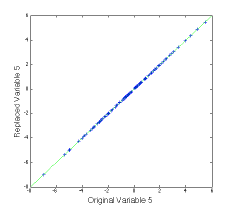
We can try R_m out on a new data set that spans the same space as the previous one, and plot up the results as follows:

>> newx = randn(100,5)*p’;
>> var5 = newx(:,5);
>> newx(:,5) = 0;
>> newx_r = newx*Rm;
>> figure(2)
>> plot(var5,newx_r(:,5),’+b’), dp

The (not very interesting) figure at left shows that the replaced value of variable 5 agrees with the original value. This can be done for multiple variables.

In the second installment of this Missing Data series I’ll give some examples of how this works in practice, discuss limitations, and show some alternate ways of estimating missing values. In the third installment we’ll get to the much more challenging issue of building models on incomplete data sets.

BMW

B.M. Wise and N.L. Ricker, “Recent advances in Multivariate Statistical Process Control, Improving Robustness and Sensitivity,” IFAC Symposium n Advanced Control of Chemical Processes, pps. 125-130, Toulouse, France, October 1991.